Author: Guoping Zhao, Lauflabor (www.lauflabor.de), TU Darmstadt, Germany

Date: July, 2019

This wiki shows how to build a Hill-type neuromuscular model in simulation.

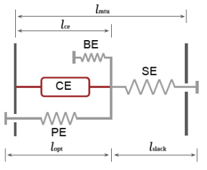
Figure 1: Muscle-tendon unit (MTU) model. CE, BE, PE and SE denote contractile element, buffer elasticity, parallel elasticity, and series elasticity, respectively.

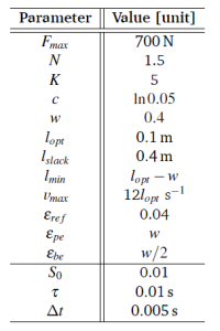
The Hill-type muscle-tendon unit (MTU) model (Geyer2010) is used in this paper. The MTU consists of a series elasticity (SE), a contractile element (CE), a parallel elasticity (PE), and a buffer elasticity (BE). The generated CE force $F_{ce}$ is computed by the muscle activation ($A$), maximum isometric force $F_{max}$, force-length ($f_l$) and force-velocity ($f_v$) relationships of the CE (Geyer2010, Geyer2003): \begin{equation} \label{eqn_fce} F_{ce} = A F_{max} f_{l}\left(l_{ce}\right) f_v\left(v_{ce}\right) \end{equation} \begin{equation} \label{eqn_fl} f_{l}\left(l_{ce}\right) = \exp\left(c\left| \frac{l_{ce}-l_{opt}}{l_{opt}w} \right|\right) \end{equation} \begin{equation} \label{eqn_fv} f_{v}\left(v_{ce}\right) = \left\{ \begin{array}{lr} \frac{v_{max}-v_{ce}}{v_{max}+Kv_{ce}} & v_{ce} < 0\\ N + \left(N-1\right) \frac{v_{max}-v_{ce}}{7.56Kv_{ce}-v_{max}} & v_{ce} \ge 0 \end{array} \right. \end{equation} where negative CE velocity $v_{ce}$ denotes the concentric movement. The width $w$ and residual force factor $c$ define the shape of $f_l$. The eccentric force enhancement $N$ and the shape factor $K$ define the $f_v$. The MTU force $F_{m}$ can be computed as \begin{equation} \label{eqn_fmtu} F_{m} = F_{se} = F_{ce} + F_{pe} - F_{be} \end{equation} where \begin{equation} \label{eqn_fse} F_{se} = \left\{ \begin{array}{lr} F_{max} \left(\frac{l_{se}/l_{slack}-1}{\varepsilon_{ref}}\right)^2 & l_{se}>l_{slack} \\ 0 & l_{se} \leq l_{slack} \end{array} \right. \end{equation} \begin{equation} \label{eqn_fpe} F_{pe} = F_{max}\left(\frac{l_{ce}-l_{opt}}{l_{opt}\varepsilon_{pe}}\right)^2 \end{equation} \begin{equation} \label{eqn_fbe} F_{be} = F_{max}\left(\frac{l_{min}-l_{ce}}{l_{opt}\varepsilon_{be}}\right)^2 \end{equation} where $l_{se}$ is the SE length, $l_{slack}$ is the SE rest length, $\varepsilon_{ref}$ is the reference strain of the SE, $\varepsilon_{pe}$ is the reference strain of the PE, $l_{opt}$ is the optimum length, $l_{min}$ is the BE rest length, $\varepsilon_{be}$ is the BE reference strain All the parameter values are listed in the following table.

The muscle excitation-contraction coupling (ECC) is modelled as (Geyer2003): \begin{equation} \label{eqn_ecc} \tau \frac{\mathrm{d}A(t)}{\mathrm{d}t} = S(t) - A(t) \end{equation} where $S(t)$ is the stimulation signal (neural input), $A(t)$ is the muscle activation, and $\tau$ is a time constant. We assume a linear relation between $S$ and the sensory feedback $P$ (i.e. $F_{m}$, $l_{ce}$, $v_{ce}$): \begin{equation} \label{eqn_stim} S(t) = \left\{ \begin{array}{lr} S_0 & t \leq \Delta t \\ S_0 + GP(t-\Delta t) & t > \Delta t \end{array} \right. \end{equation} where $S_0$ is the constant stimulation bias, $G$ is the gain factor for different feedback signals, and $\Delta t$ is the sensory feedback time delay. $S(t)$ is saturated in the range of $[0, 1]$. In the implementation, each sensory feedback $P$ signal (i.e. $F_{m}$, $l_{ce}$, $v_{ce}$) is normalized. More specifically, $S(t)$ for each individual feedback pathway (i.e. force feedback (FFB), length feedback (LFB), and velocity feedback (VFB)) is computed as: \begin{equation} \label{eqn_stim_fb} S(t) = \left\{ \begin{array}{lr} S_0 & t \leq \Delta t \\ S_0 + G_F F_m^n (t-\Delta t) & \text{FFB}, t > \Delta t \\ S_0 + G_L l_{ce}^n (t-\Delta t) & \text{LFB}, t > \Delta t \\ S_0 + G_F v_{ce}^n (t-\Delta t) & \text{VFB}, t > \Delta t \end{array} \right. \end{equation} where $F_m^n = F_m/F_{max}$, $l_{ce}^n = l_{ce}/l_{opt}$, and $v_{ce}^n = v_{ce}/v_{max}$. $G_F$, $G_L$, and $G_V$ denote the gain for force, length, and velocity feedback pathway, respectively.

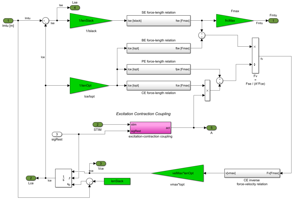
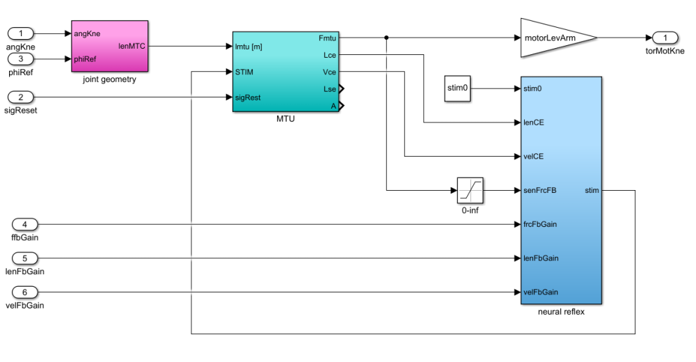
According to the Hill-type muscle equations, we build the MTU model with Matlab simulink (Geyer2010).

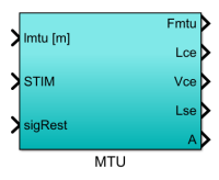
The input of the MTU model is the length of the MTU (lmtu), muscle stimulation signal (STIM), and the rest signal (sigRest, rest the integrator when the system state changes (e.g. from flight to stance)). The output signals are the MTU states including muscle force (Fmtu), muscle length (Lce), muscle velocity (Vce), tendon length (Lse), and muscle activation (A).

Here's the overview of the simulink model which calculate knee joint torque based on joint angle.

With the virtual muscle states from the MTU block, muscle stimulation signal is computed based on the linear combination of muscle force, length and velocity reflexes.